Data Considerations
Portfolio can consume Opportunity Input data, Attributes, and basic Selection Rules from Excel, Enersight, and Planning Space data sources. Selection Dependencies and Groups may be configured using attribute variables and imported directly from Planning Space modules. The user can export all Selection Rules from Portfolio to further refine them in Excel. Model Expressions and Metric Constraints must be imported using Excel.
In this section, we will first discuss the Opportunity Input Data, Attributes, and Selection Constraints. These three types of data are necessary in order to create a portfolio. Next, we will discuss Master Data and Selection Dependencies. Master Data and Dependencies can be imported intoPortfolio as needed, but they are not necessary to create a portfolio.
Finally, we will cover Metric Constraint data, which is imported into a particular Scenario rather than into the portfolio as a whole.
We will cover Expressions in detail in the Modeling section that follows.
ep Input Data Tab
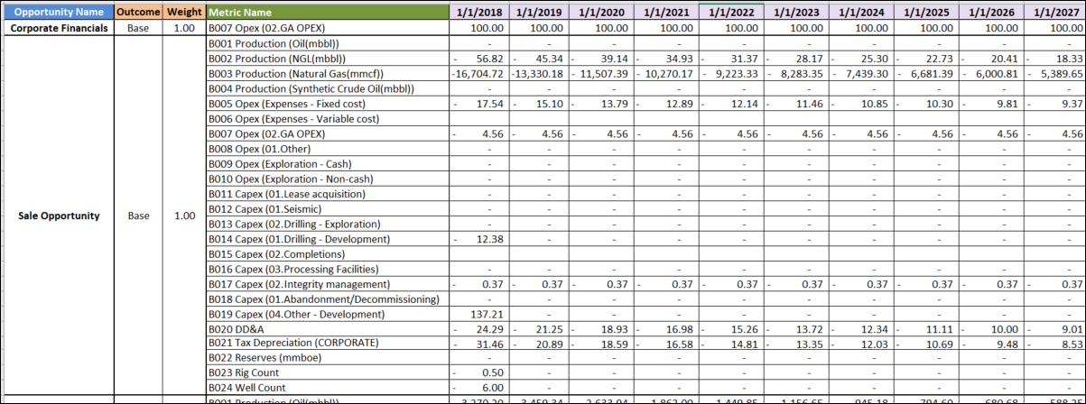
Below is a typical Excel format for Input Data, found on the “ep input data” tab of the Excel template mentioned above.
Input Data, or time series data, constitutes a forecast of how a specific Opportunity will behave if chosen for investment. For example, choosing to invest in an Opportunity will require a series of capital outlays, and, with luck, will result in a production stream with related operating expenses, taxes, and so forth. If the Outcome of an investment is uncertain, we provide a number of Outcomes for each Opportunity to better capture this uncertainty.
In the ep input data tab, data is organized into Opportunities (Column A). Each Opportunity may have one or several Outcomes (Column B), each with a weight (Column C). Each Opportunity has a number of Metric names (Column D), followed by time series data associated with those Metrics (column E through the end of the set).
Click image to expand or minimize.
Each Opportunity need not contain all of the Metrics listed on the sheet (for instance, see the “Corporate Financials” Opportunity at the top). However, it is necessary to fill all the data cells, even if we simply fill zeros where appropriate.
ep Attributes Tab
The ep Attributes tab contains Attributes and their corresponding characteristics. Once we import this data, we will find these Attributes and Characteristics in many Portfolio views. Attributes are broad categories that apply to the entire portfolio. Characteristics are the alphanumeric descriptors of Opportunities that belong to each Attribute.
Attributes allow us to:
- Filter within Portfolio and group similar Opportunities.
- Create Expressions that apply only to a limited set of Opportunities.

Click image to expand or minimize.
Each Attribute appears in a column heading at the top of the table (in this example, Country, Region, Region-Detail, and Field). Characteristics are the data filling the intersections of Opportunities and Attributes. For example, the Characteristic for Opportunity 2, Attribute “Region,” is “Canada.”
Note that these Opportunity names must exactly match the Opportunity names used in the ep input data tab.
“Fixture?” is a special Attribute name used to designate Master Data, which will be discussed in more detail later.
ep Selection Constraints Tab
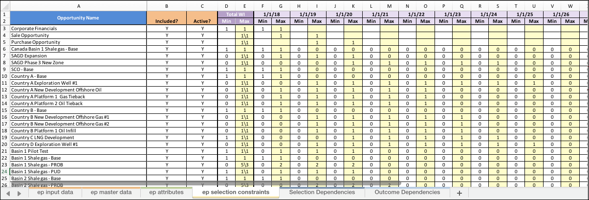
Selection Constraints tell the portfolio how many Opportunities it may choose and when it may choose them during optimization. Below is an example of the Selection Constraints portion of a source file.
Click image to expand or minimize.
In this part of the file, we can
- Define the time periods during which an Opportunity can be scheduled, usually in years.
- Define Selection Min and Max for a given Opportunity, both for all years in consideration (Total) and for each individual time period. Either or both may be left blank. If there is a Min, the corresponding Max must be equal to or greater than it. A blank (or zero) for a Max means that no selections are allowed during that time period.
- Choose whether an Opportunity’s selection is subject to instance selection or not. While there are no columns for Instance Max and Min in the Input file, we can specify Instance Max by entering it after a slash in the Total Max column (see column E above). When the Instance cells are populated, a fractional selection counts as an entire instance. If multiple selections are allowed in the time period, those selections are rounded up to the nearest integer for evaluation against the instance count.
- Choose whether an Opportunity is active or not. This feature is not yet enabled. To disable an Opportunity, set both the Total Max to zero.
Comments on Importing Data
- Opportunity names must be unique.
- Opportunity names in the Input Data, Attributes and Selection Constraints tabs must match each other.
- We may add as many Outcomes to a given Opportunity as needed.
- Metrics may differ from one Opportunity to another.
- Different Opportunities may have different numbers of potential Outcomes.
- The Metric names that esi.manage and Enersight use when generating data can be changed in the Expressions file by referencing the data in the old Metric from our new, preferred Metric name. Upon doing so, that new name becomes a Computed Metric.
- If we want to import data from several files into an existing portfolio, the import will use a replace, not append, strategy. Therefore, we want all the Selection Constraints in one file, even if the rest of the data is in separate files.
- Always check the imported data in Portfolio before undertaking an analysis, especially if several other recent imports have been performed.
- The time periods defined in the Selection Constraint tab must be in Excel date format.
The following sections discuss Excel tabs that are optional for upload. Neither Master Data nor Constraints are necessary to create a portfolio, but both will extend our analyses.
ep Master Data Tab
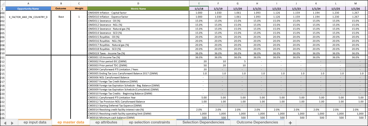
Master Data is data that does not move in time, but that can have different values in different time frames. Master Data is quite useful in Expression writing, as we will discuss in the Expressions section of this manual.
The ep master data tab is constructed much like the ep Input Data tab. Data is grouped into “Opportunities.” These Opportunities have “Metrics” (the Master Data) and are assigned to actual Opportunities via Attributes.
For example, if three regions have three different tax rates, we can simply write an Expression like “Net Production x Tax Rate.” Portfolio will decide which tax rate goes with which Opportunity by determining which Opportunities have common “Region” Attributes. We will discuss this concept in greater detail in the Modeling section of this manual.
Click image to expand or minimize.
Creating Master Data requires a few steps:
- Populate the ep master data tab.
- Add the Master Data “Opportunity” names to an ep attributes tab.
- Set the Attribute called “Fixture” to “Y” for the Opportunities that contain Master Data.
- Assign the Master Data Opportunities to other Attribute/Characteristic pairs (it is usually best to assign a Master Data Opportunity to only one Attribute).
No action is required in the ep Input Data tab or the ep Selection Constraints tab.
Things to Consider
In the example below, we only want “Master Data Canada” to apply to Opportunities with a Characteristic of “Canada” for Attribute “Country.”

Click image to expand or minimize.
Master Data matches using a cascading logic. When seeking a match between an Opportunity and Master Data, Portfolio will work its way from the top to the bottom of the Master Data Opportunities, as listed on the Attributes tab. If it finds a match (for example, both the Opportunity and the Master Data Opportunity have the Characteristic “USA” under the Attribute “Country,” without any conflicting Attributes), it will take that match. If it does not find a match, it proceeds to the next Master Data Opportunity in the list.

Click image to expand or minimize.
We can take advantage of this structure to match different Master Data to different Attributes at different granularities. For example, there could be a match for Asset, which comes before a match for Region, which comes before the match for Country. An Opportunity will have Characteristics for all three Attributes but will match the more specific (or more granular) level first if that level is first in the Attribute list.
It is best practice to have a “Default” Master Data Opportunity at the bottom of the list, with no Attributes listed except for “Y” under “Fixture?” The data in the Master Data default Opportunity will match anything that hasn’t found a match above.
Note that the total number of time periods listed for the Master Data Metrics should equal the number of selection time periods (from the Selection Constraints), plus the maximum number of time periods listed for the Opportunities, minus one. For instance, if you select a project in year 10 and it has 20 years of data, its data will begin in year 10 and end in year 29.
Scenario-Level Master Data
Master Data can be held either at the portfolio level or at the Scenario level. Most Master Data is held at the portfolio level. If it is held at the Scenario level, we can choose among different Scenarios from within the Active Scenario view in the Details tab.
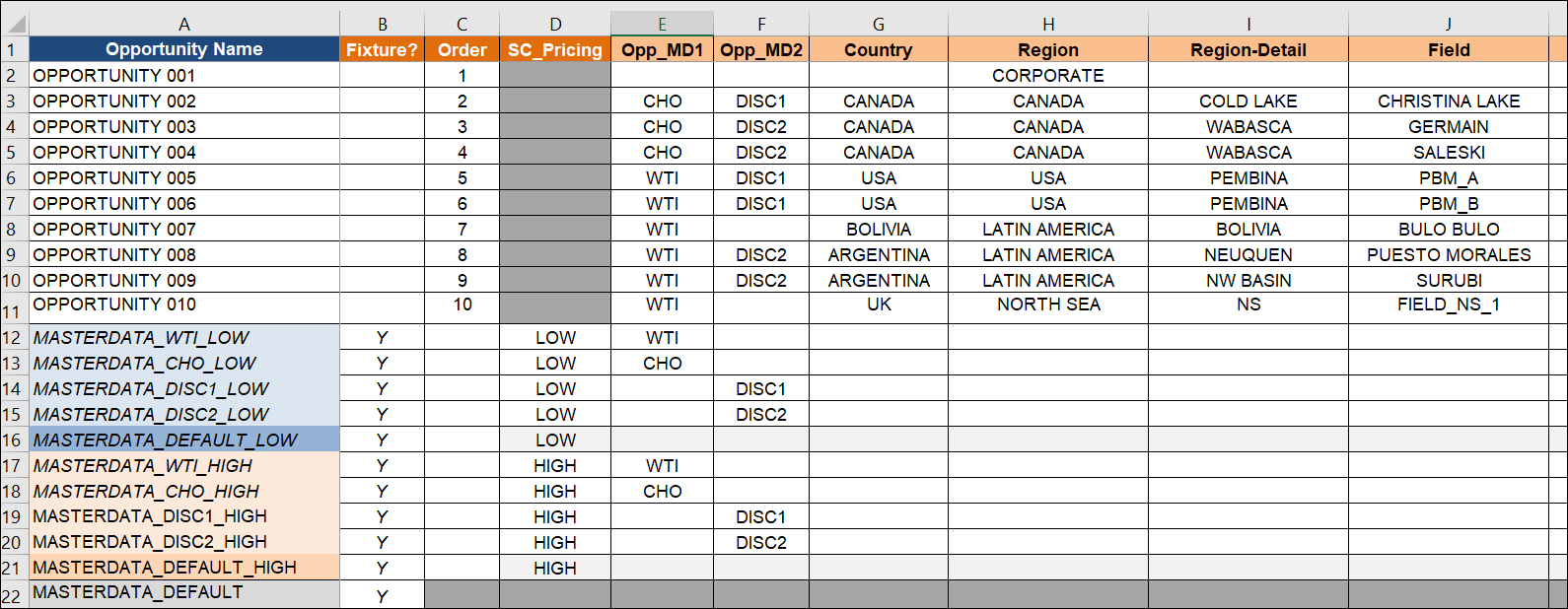
A common example is oil or gas price. We often want to compare different Scenarios at different prices. In order to do this, we create Master Data Opportunities that contain the different prices (e.g., High, Base, and Low) and designate them with an Attribute that is not used to describe any of the “normal” Opportunities. The fact that the new Attribute is not associated with any regular Opportunities is a signal for Portfolio to treat them as Scenario Attributes. It is good practice to put the name “Scenario,” or something similar, in the Attribute name. In the example below, SC_Pricing is the Scenario Attribute. Note that it is not used for any of the Opportunities above it, which are grayed out.
Click image to expand or minimize.
Dependencies
Dependencies define relationships among Opportunities and may affect how Selections are made during optimization. In the Selection Dependencies and Outcome Dependencies sections that follow, we will use two Opportunities and the Dependencies that are based on them to demonstrate how Dependencies work.
Selection Dependencies
Selection Dependencies describe how the select-ability of one Opportunity (Dependent) depends on the selection status of another Opportunity (Independent). For example, one Opportunity may be an exploration/experimental project, while another Opportunity may be the development project associated with the first. We would obviously need the exploratory project to occur before the development project, so we would need to write a Selection Dependency that specifies when such a project should be chosen.
In this example, we will treat Opportunity 2 as if it were an exploratory project and Opportunity 3 as if it were a development project. We need Opportunity 2 to occur before Opportunity 3, so we write a Dependency that indicates that (see image below).

Click image to expand or minimize.
Let’s define the columns in the Selection Dependencies tab and what they indicate in this example:
- Active? – This column determines whether a Dependency is active in the model. Both rows have a “Y” (for yes) listed, so both are active here. We can toggle a Dependency on and off using this column.
- Independent Opportunity – The Opportunity listed in this column is used in the first part of the Dependency logic. In this example, Opportunity 002 must occur before Opportunity 003, meaning that Opportunity 003’s timing relies on the fact that Opportunity 002 occurs first.
- Must/Must Not – This column is used to indicate the relationship between Opportunities. If it says Must, then the dependent Opportunity can’t be chosen unless the independent Opportunity is chosen as well. If it says Must Not, then the opposite is true: if the independent project is chosen, then the dependent project can’t be chosen. For example, in the second line of the illustration above, Opportunity 5 and Opportunity 6 are mutually exclusive. If Opportunity 005 is chosen, Opportunity 004 must not be chosen. We might use this function if we have two potential Opportunities in the same region, but only one can be chosen.
- Time Period Offset – A time period offset is used to determine how two projects interact with each other in time. For example, if the time period offset were -2, the independent project would have to occur 2 or more time periods before the dependent project is allowed.
- Before/After/During – This column determines whether an independent project must occur before, during, or after the dependent project. During means in that time period only, while Before and After mean any time up to or beyond that that time period, inclusive.
- Dependent Opportunity – This is the Opportunity whose selection depends on whether the independent Opportunity is selected.
- Each # N/R Dependent OpportunityandNeed # N/R Independent Opportunity– Defines the ratio of dependent Opportunities that can be selected as a result of independent Opportunity selection. In this example, Opportunity 003 may be selected two times for every one time that Opportunity 002 is selected.
- N/R- N = Natural number (instance count). R = Real number (interest). The number of instances in each time period is equal to the selection quantity, rounded up to the nearest whole number. The total instances in all time periods is used to evaluate the dependency. Interest (R) is the actual sum of all selections whether partial or whole.
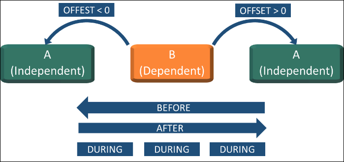
Click image to expand or minimize.
Mutual Groups
Mutual Groups are a simple way of configuring how an Opportunity can or cannot be selected, depending on the selection status of other members in a group.
Mutual Exclusive Group
In the example below, 3 different development strategies for a program are considered. Any one of the strategies may be selected, but only one.
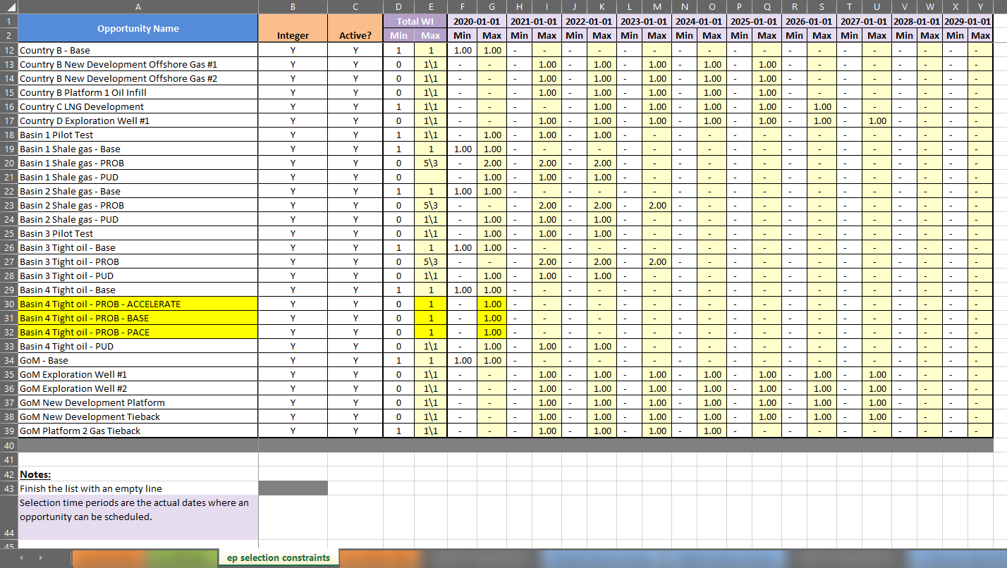
Click image to expand or minimize.
In this case we can add the 3 possibilities to a Mutually Exclusive Group, whereby if one Opportunity is selected the other group members cannot be selected.

Click image to expand or minimize.
The selection of any of the 3 is dependent on the optimization strategy configured in a Scenario, but only one will ever be selected. For example, the accelerated tight oil may be selected for maximizing oil production in earlier time-steps, while the paced option may be selected for maximizing oil production in later time-steps.
Mutual Inclusive Group
In the example below, 2 different corporate level elements are modeled. Generally, with Inclusive Groups, any one of the strategies may be selected, but if one is selected in a time-step then both are. Specifically, in this case the Corporate Financials are required in Year 1 but the Sale Opportunity may be selected in Years 1 or 2.

Click image to expand or minimize.
In the example inclusive group however, the Sale Opportunity is forced to be selected along with the Corporate Financials and in the same time step.
If the group is disabled in a Scenario, the Sale Opportunity may or may not be selected in any of years it is included in the constraints table above.

Click image to expand or minimize.
Outcome Dependencies
Outcome Dependencies are used to relate the Outcomes of two Opportunities to one another. Outcome Dependencies allow us to alter how the dependent Opportunity behaves during Monte Carlo simulation, depending on which Outcome is chosen for the independent Opportunity.
Outcome Dependencies behave in two ways, outlined below.
During a Monte Carlo simulation, when the independent Opportunity Outcome chosen is one that triggers a reaction in the dependent Opportunity, the dependent Opportunity will respond accordingly. This will be reflected in the Monte Carlo results.
However, when we are optimizing, we are not running a Monte Carlo simulation. Instead, we are using Outcome weights to calculate expected values, so we optimize using expected values to find the best set of selections that meet our selection criteria. If we create an Outcome Dependency that says, for example, that the dependent Opportunity will only go forward if the independent Opportunity is successful, and the success Outcomes for the independent Opportunity carry a weight of 50%, then the expected value of the dependent Opportunity will be reduced by 50% to reflect the fact that it will only be chosen in half of the possible Monte Carlo scenarios.
It might seem that, if one Opportunity is conditionally dependent on another and the independent Opportunity is chosen during optimization, then the dependent Opportunity must be chosen as well. This is not the case. An optimization may choose not to select either project. To ensure a relationship between Opportunities, we must include Selection Dependencies, as well.
For example, we might say that an appraisal Opportunity can only occur if a discovery (the exploration Opportunity) occurs first. This Dependency only governs the value of the dependent Opportunity.
If we also want to say that the independent Opportunity must be chosen at least one year before the dependent Opportunity, or that the dependent Opportunity must be selected if the independent Opportunity is successful, that would require a Selection Dependency.
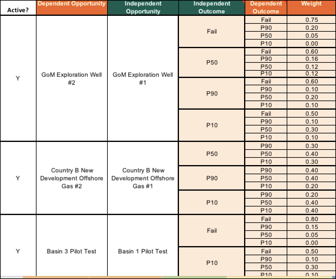
Click image to expand or minimize.
To set up an Outcome Dependency, use the template provided and follow these instructions.
- Indicate a dependent Opportunity in the Dependent Opportunity column.
- While we can rearrange the columns, we should keep them in a logical order, ensuring that when we move a heading, we move its corresponding data, as well.
- Next, enter the name of an independent Opportunity into its column.
- While the independent Opportunity can repeat (or have a max selection of more than one), the Dependency will be based on the first selection of the independent Opportunity.
- Because of this, we recommend that the independent Opportunity not repeat in all but some special cases.
- Place the independent Opportunity’s Outcomes that will trigger a response in the dependent Opportunity in the independent Outcome column above.
- We can list all these names in the same cell and merge them to correspond to the dependent Outcome meant to be tied to them, or
- We can repeat the list ("Base” and “High" in the figure below) in each cell that corresponds to a dependent Outcome.
- An asterisk (*) in the Independent or Dependent Outcome columns denotes "all outcomes not listed above." This logic is resolved on import.
- Finally, enter the name of the dependent Outcome and the weights that will result if the independent Outcome occurs into their appropriate columns.
- The column "If the independent Opportunity does NOT have one of the target Outcomes, then:" is descriptive only. It allows us to indicate the result of the situation set up in the previous columns.
This process can be confusing, so let's go through some examples. The first row in the illustration below can be read as follows: If, during a Monte Carlo simulation, Opportunity 2's Outcome ends up as either the Base Outcome or the High Outcome, then Opportunity 3 can go ahead at the weight specified. However, if Opportunity 2's Outcome ends up at any other Outcome (*), then Opportunity 3 cannot go forward (the weight for the * outcome is 0.0).
Similarly, the example in the third row can be read as follows: when Opportunity 2's Outcome is “Base” or “High,” Opportunity 3 will have an outcome of "Base." If Opportunity 2's Outcome is anything else (*), any of Opportunity 3’s Outcomes can be chosen using the weights listed in the “Weight” column.

Click image to expand or minimize.
For the expected value calculation in the first example, we give the asterisk a weight of zero to represent a null (no Opportunity chosen) if any outcome other than Base or High is chosen.
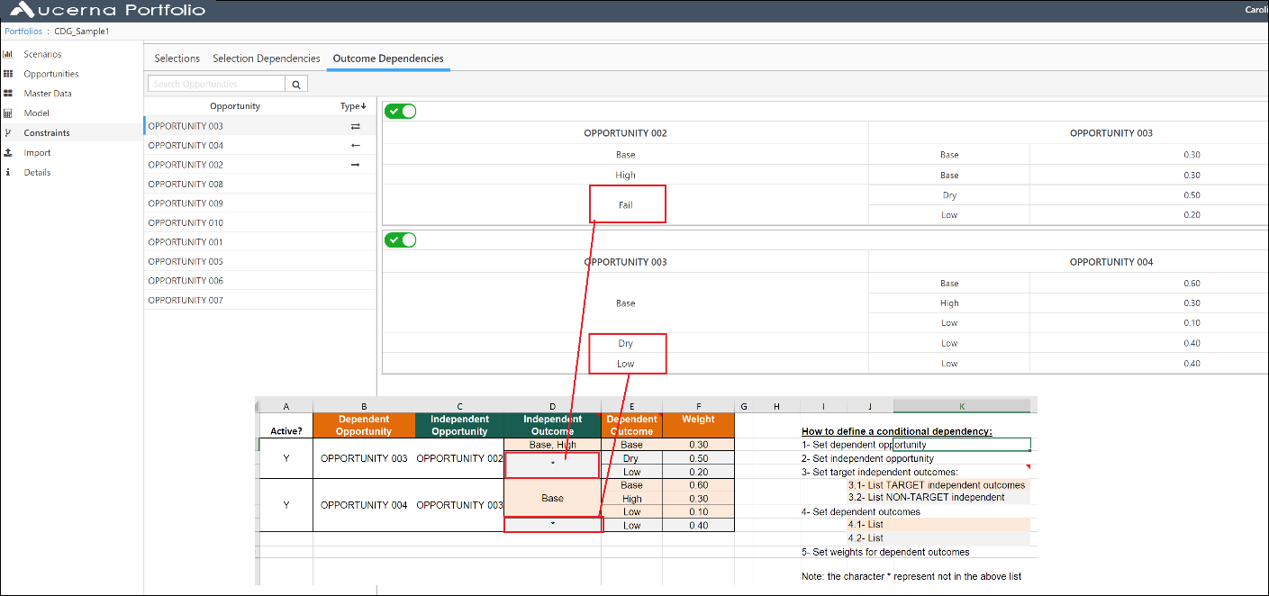
Click image to expand or minimize.
Therefore, the expected value accounts for the probability that the Outcome Dependency may go in one direction or another, while the Monte Carlo simulation will recognize the full range of possible Outcomes based on the Dependency. Note that the subsequent reduction in value in the expected value case will not appear in any of the Opportunity views. However, it will be evident in the pertinent calculations.
Please note:
- The independent Opportunity should not be a surrogate; that is, it cannot have a Total Max of >1 in the ep selection constraints tab.
- The Conditional Dependency will cause a reduction in the expected value of the dependent Opportunity that will be used during optimization; however, the full value of the various Outcomes will be used during Monte Carlo simulation.
- We can adjust dependent Outcome weights based upon what happens in the independent Opportunity.
Metric Constraints File
There are two methods for setting Metric Constraints: using the Metric Constraints tab in Scenario view or importing a Metric Constraints file from Excel. This section discusses the structure of a Metric Constraints file from Excel.
The Metric Constraints file is used to upload Constraints, or targets, into a scenario. These Constraints can apply to either Input or Computed Metrics. The column headings are as follows:

- Metric Name – Note that this name must exactly match the Metric name listed in the Expressions file and/or Input file.
- Enforce? – Values are always loaded, but are only active if Enforce?=Y. We can toggle Enforce? to test different Constraints in different Scenarios.
- Type – Min or Max.
- Default – Value for every instance in the time series if the time cell is not populated or the value in the case of an indicator.
- Remaining cells – The rest of the cells have a time or date in the heading. These cells contain the Constraints that correspond to each time period.
