
Perfect Communication
Introduction
In PetroVR the user describes the performance of individual wells by means of decline and injection curves. Those curves represent the ideal behavior that the wells would exhibit under ideal conditions. Separately, the user specifies the capacities at which facilities can operate, and depicts the diagram that interconnects wells and facilities with pipes that let the fluids flow thru the system.
The aim of the simulation is to let the user understand how the wells would produce (or inject) under the constrained conditions of a system made up from parts that have physical limits.
The dynamic nature of the model makes of its predictability a non trivial problem. As new wells are drilled and old ones are exhausted, the conditions may change radically. Different factors impact the development of the system as the unavailability of rigs, the expansion of facility capacities, or the application of external stimuli as the ones produced by gas-lift equipments or gas compressors.
As originators of all such interactions, performance curves attain special significance. In that regard a direction on which the system could extend its flexibility is by modeling the way in which the wells that belong to the same reservoir communicate each others. The membership to the same reservoir entails bounds that complement those derived from user defined interconnections. The explicit support of well intercommunication should help engineers to better describe the ideal conditions at which wells would operate, had all physical constraints be removed. This document describes the new functionality under the extreme premise of perfect communication. A more realistic approach, in which the communication between wells is partial, is briefly discussed in a subsequent section.
Modeling Perfect Communication
Consider the reservoir as a tank. At any given moment there are a number of active wells attached to it. Some are producers, others are injectors. Assume that the total reserves are known and that the potential overall production can be described by a dimensionless table as follows:
| Cum % | Rate % |
|---|---|
| 0.0 | 100 |
| 10 | 85 |
| 20 | 70 |
| 30 | 60 |
| 40 | 55 |
| 50 | 50 |
| 60 | 45 |
| 70 | 40 |
| 80 | 35 |
| 90 | 15 |
| 100 | 01 |
The table establishes that the reservoir starts producing at a certain rate. Afterwards, when say 30% of the reservoir reserves have been produced the rate drops down to 60% of that initial potential. Finally, when all the recoverable fluid has been exhausted, the reservoir is abandoned at 1% of the initial rate.
Now assume we are at a point of time where the reservoir has produced some amount of barrels. The question we must answer is how much each of its wells would produce the next day.
Of course, not all the producers have the same potential. For instance, if the reservoir has three wells, then we could have the following configuration:
| Well | Initial Rate |
|---|---|
| A | 200 bpd |
| B | 500 bpd |
| C | 300 bpd |
Say that the total amount of recoverable fluid of the reservoir is 10 millions of barrels. Had the three wells start producing the first day, they would contribute with an initial rate of 1000 bpd. Those two quantities could be used to dimension the reservoir decline table.
We could use the initial rate of the wells as the indication of their relative potential. In doing that it is reasonably to expect that Well A would produce at 20% the rate of the reservoir, Well B 50% and Well C 30%.
| Well | Contribution |
|---|---|
| A | 20% |
| B | 50% |
| C | 30% |
Going back to the moment when the reservoir has produced some amount, say 2 millions of barrels, we deduce that such production corresponds to 20% of the total reserves, which in turn gives a rate of 70% of its initial potential according to the first table. Since the three wells would produce 1000 bbl the very first day, our expected production for tomorrow is 700 bbl. That in turn represents 20% of 700 = 140 bbl for Well A, 50% of 700 = 350 for Well B, and 30% of 700 = 210 for Well C.
After that day, the cumulative production of the reservoir would be 2,000,700 bbl. By entering again in the table with the percentage corresponding to the new value of cum, we can now compute a new rate percent. As before we find out the production of that day and then prorate it among the wells using the contribution table.
A similar analysis applies to injectors. If the injection curves relate cumulative production percents with injection rates, then we could follow the same approach to calculate the amount of injection for tomorrow based on the cumulative percent of the reservoir today.
More on Injection
The description above explains how to compute the potential production of the wells today based on the cumulative production of the whole reservoir yesterday. To find out the injection rate we would proceed, in principle, in a similar way. The only detail to keep in mind is that, since injection rates are based on the cumulative production, we must first find out the production of today and then use the injection decline to calculate the corresponding injection.
For instance, assume that the reservoir has produced 60% of its reserves. We first compute the production for today. Say that such a production represents 0.02% of the total reserves. To find out the corresponding injection rate we enter the injection curve with two values 60% and 60.02%. Since the injection curve specifies dimensionless injection rates in terms of dimensionless cumulative production, we can interpolate that table to get the corresponding injection percentages. Let's call those to two dimensionless injection rates q0 and q1. We don't know exactly how the injection rate must evolve from the first rate to the second. So we approximate that behavior by averaging the two values. In other words, we use the mean q = (q0 + q1) / 2. Now we can compute the actual injection rate of each of the wells by multiplying the quantity q just calculated by the initial injection rate of the wells.
The Dynamics of Perfect Communication
From the viewpoint of the simulation, the scenario depicted above only considers the problem instantaneously, that is, while the simulation timer ticks by one single step. In a broader perspective we must also take into account the fact that as new wells are drilled and older ones are exhausted, the configuration of the reservoir changes. This has some impact on the implementation; for instance, we cannot pre-compute the relative contributions of the wells in advance, as the wells involved may change from one step to the other. It must be understood that, under the perfect communication hypothesis, the production (or injection) rate of one well depends on all other wells that are active in the reservoir.
It must be also observed that the simulation does not necessarily step day by day. It usually jumps in longer periods to achieve a better computation speed. However, the simulation only jumps over periods where no events can happen. In particular, within a jump of some number of days it is guaranteed that no wells will become on-line or will be abandoned. As a result, the configuration of the reservoir remains unchanged during the jump, and our local analysis remains valid.
Understanding the Consequences
With perfect communication the behavior of the individual wells might, at first glance, look counterintuitive. For instance, with any usual decline curve where the rate of the well depends on the cumulative production of itself it is expected for the well to start producing (or injecting) at its initial rate. That simple fact may not be true with perfect communication. When a new well is drilled and acquires the on-line status, its performance will be the one that corresponds to the cumulative production of the reservoir.
In the example above assume, for instance, that Well A becomes on-line when the reservoir has produced 60% of its reserves. At that point the decline curve of the reservoir has a potential rate of 45%. Then, Well A will start producing at 200 bpd x 45% = 90 bpd, even though the user specified an initial rate of 200 bpd for it. In other words, the actual initial rate might be considerably lower than the one specified by the user. Had the well become on-line the first day the reservoir starts producing it would exhibit the "ideal" initial rate the user defined, otherwise it won't. This could be interpreted as a change in the meaning of the initial rate. Without perfect communication all wells will start with the potential of their initial rates; with perfect communication most wells will start, most likely, at a lower performance.
Explicit Assumptions
The reasoning behind our approach makes some assumptions that must be explicitly enounced. We have said that our physical model for a perfectly communicated reservoir is that of a tank. As such the reservoir has an intrinsic dimensionless decline curve that determines how its production performance would decay as its reserves are exhausted. In that physical model a well is thought as a perforation in the tank.
The instantaneous rate of the fluid going out thru that perforation depends on two parameters. One is the location of the hole. The other one is its section (area). The greater the section, the faster the fluid escapes. The deeper the location, the greater the pressure at that point.
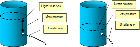
Those two physic characteristics, location and section, are enough to determine the instantaneous escaping rate of the perforation. Thus, in this simplified model, the potential of the perforation depends on its location and its area.
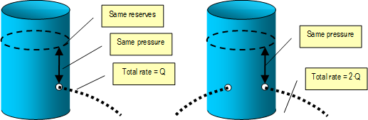
If a second perforation is drilled, then the two individual rates would be summed up, and the reserves would be exhausted faster. In consequence, the pressure at any location would decrease faster.
In this model, the initial rate of a perforation is defined as the rate the fluid would escape the perforation, had the tank contained its full reserves. The rate at any other level of reserves can be calculated from the dimensionless decline curve and the cumulative production corresponding to that level (that is, the difference between the initial and the actual reserves of the tank).
It is worth noticing that the initial rate of a well captures its potential the same as the location and section of the hole would capture the potential of a perforation on the tank.
Unknown Reserves
Another difference between the isolated model and perfect communication is that in the first one the initial reserves of each of the wells are known beforehand. With perfect communication that quantity remains unknown until the well stops producing. In this case the wells will be abandoned when their rates fall below the economic limit, or when the reservoir has exhausted its reserves. In other words, with perfect communication well reserves are unknowns that the simulation finally solves.
The fact that well reserves are found out at the end impacts on other parts of the system. For instance, the system can no longer auto-deplete a reservoir the way it did before. Given that well reserves are unknown beforehand, there is no way to calculate how many times the initial pattern of producers and injectors must be cloned. The user can still indicate the system to auto-deplete a reservoir by providing the total number of wells to be drilled in that development.
Perfect communication also impacts on infill drilling. In the isolated case the user must tell the system how the infill will affect the reserves of existing wells. That specification is no longer possible or necessary. Since the performance of any well is already dependent on all active wells in the reservoir, any infill drilling will affect the performance of the other wells.
In the case of gas reservoirs that use pressure-dependent decline curves such as deliverability or quadratic declines, the property of perfect communication is supported in such a way that the pressure of the reservoir is equilibrated.
The action of decline switching makes no sense when the reservoir has perfect communication. Such action is intended to change a well decline with another; consequently it is not applicable when all the wells obey the same reservoir decline.
Finally, being the well reserves found out at the end makes it impossible to book well reserves in that way.