On Gas Injection Modification

Introduction

When gas (or water) is injected into a reservoir, the actual performance of its wells is modified in a given way. Performance curves in PetroVR are specified so as to define the ideal behavior of the wells when producing in isolation. Therefore, changes in the performance derived e.g. from injection need to be simulated dynamically by taking into account the actual evolution of the system. In particular, the impact of injection on production needs to be modeled in terms of the volume injected and the oil produced.

This section explains the algorithm devised for the dynamic adjustment of the potential production based on injected gas, and its implementation in PetroVR. Given that it is used for perfectly communicated oil reservoirs, the reader should be familiar with the Perfect Communication section.

Definitions

The swept oil PV fraction (SOPVF) is the quotient of gas injected into the reservoir divided by the hydrocarbon pore volume (HCPV) of the reservoir, and modified by the formation volume factor (Bg - ratio of volume of gas at reservoir conditions to that of surface conditions). In consequence, the ratio is a dynamic quantity that changes as the simulation runs.

In this section reservoir is understood as an oil reservoir with perfect communication among all its wells, that is, injection and performance curves are dimensionless descriptions of the behavior of the reservoir as a whole. The current implementation of PetroVR only supports the Table Performance Type type.

The recovery factor is the usual PetroVR parameter used to determine the amount of fluid that can be produced by the reservoir.

Injection Modification Table

This table specifies the relationship between the gas injection ratio and the recovery factor and performance and injection curves of a reservoir's wells. Here is an example:

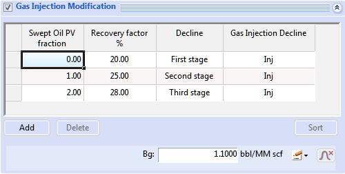
Intermediate values of the fraction, not explicitly defined in the table, are computed by linear interpolation. For instance, assume a given value r of the fraction lays between the values in lines i and i + 1 in the table. Let's call those two ratios r_i and r_i+1. We compute the interpolation coefficient λ such that:

r = λ r_i + (1 - λ) r_{i + 1}

Next we can compute the recovery factor corresponding to r using the recovery factors at lines i and i + 1 as follows:

rf = λ rf_i + (1 - λ) rf_{i + 1}

Similarly, we can interpolate the production and injection curves at lines i and i + 1 using the same coefficient λ. Given that those curves express dimensionless rate in terms of dimensionless cum, we (only) interpolate the dimensionless rates with λ to get the interpolated curves.

Calculation of fraction and recovery factor

The algorithm proceeds dynamically by computing in each simulation step the amounts of injected (inj) and produced (prod) gas by the reservoir as a whole. Then the fraction is defined as:

SOPVF = Cum_inj * Bg / HCPV

Using the interpolation techniques explained above the algorithm computes the new recovery factor (rf) and the interpolated production and injection curves.

Once the new recovery factor rf is know, it is used to compute the updated value of recoverable fluid (oil). Basically the calculation proceeds simply as:

recoverable fluid = fluid in place * rf

From this point on, the algorithm proceeds normally using the parameters just updated. As explained under Perfect Communication, the procedure is as follows:

• The updated amount of recoverable fluid is now used to compute the new dimensionless cumulative production of the reservoir:
• dimensionless cum = cum / recoverable fluid
• The production curve is entered with the dimensionless cum just computed. The production rate q _Rread from the curve is the total potential production other reservoir for today (current step in the simulation).
• Based on the initial rates of all the producers currently on-line, a ranking factor is computed for each of them as follows: rank _w = q _0w / (Σ initial rate)
• In the formula above the initial rate q _0w corresponds to the production well w under consideration. The sum runs over all the producers of the reservoir currently on-line and adds all the initial rates of those wells.
• Now the algorithm computes the production rates of the individual wells multiplying their rank by the total rate of the reservoir computed above: q_w = q _R * rank _w
• The rate q _w is the amount of oil the well w will produce today in the current simulation step. That's how the production of each well currently on-line is determined by the algorithm.
• The algorithm uses a similar procedure to determine the amount of gas that each of the injectors currently on-line would try to inject into the reservoir. We omit the details for the sake of brevity.

However, the key point to understand how to apply the approach is to notice that the parameters modified by the table are not independent. The recovery factor impacts the way the dimensionless curves are converted to dimensional quantities. In turn, the curves provided in the table greatly impact the production and injection cumulative amounts the ratio depends on.

The mutual dependence among the inputs requires careful analysis of consistency. For instance, it might happen that at a given step the recovery factor calculated by the algorithm is invalid as it would correspond to a value of recoverable fluid less than the cumulative oil already produced. In those cases, the simulation issues a warning message and replaces the value derived from the algorithm with the nearest valid one. Since the software cannot determine whether such an inconsistency indicates incorrect input data, or it is a minor deviation with no side effect, such cases should be analyzed with care.